Example of giant height from Wood et al 2014
This is an example from Wood et al. The example aimed to use the GPRS package to replicate the Fig4A in Wood et al paper.
Get started: 2014 height data structure
The GWAS summary statistics were downloaded from the GIANT database.
Data name: GIANT_HEIGHT_Wood_et_al_2014_publicrelease_HapMapCeuFreq.txt
The data structure:
| MarkerName | Allele1 | Allele2 | Freq.Allele1.HapMapCEU | b | SE | p | N |
|---|---|---|---|---|---|---|---|
| rs4747841 | A | G | 0.551 | -0.0011 | 0.0029 | 0.70 | 253213 |
| rs4749917 | T | C | 0.436 | 0.0011 | 0.0029 | 0.70 | 253213 |
| rs737656 | A | G | 0.367 | -0.0062 | 0.0030 | 0.042 | 253116 |
| rs737657 | A | G | 0.358 | -0.0062 | 0.0030 | 0.041 | 252156 |
| rs7086391 | T | C | 0.12 | -0.0087 | 0.0038 | 0.024 | 248425 |
Which template to use?
Before starting to process the data, we have to choose which template to use. Please use the table below to select the template.
| - | chr info in the file name | chr info not in the file name |
|---|---|---|
| chr info in the header | gene_atlas_model | gwas_model |
| chr info absent in the header | gene_atlas_model | gene_atlas_model |
The chromosome information is absent in 2014 height data, and 2014 height data also has no header with Chromosome information. Thus, I choose
gene_atlas_modelas a template
Output folders
In the GPRS package, the result folder will automatically generate under the execution directory.
i.e. The user run GPRS package in /home/user/ then the default result directory is /home/user/result
The structure of output folders are:
result/plink
result/qc
result/snplists
result/stat
result/plink/bfiles
result/plink/clump
result/plink/prs
result/plink/qc_and_clump_snpslist
Step1 preparing data set - unified the data format
In step one, the filter_data function will filter raw data with p-value, the default is 1 and gives you three output files: snplist, qc'd file and summary
After preparing the data, the snplist: result/snplists/[OUTPUT_NAME].csv will be used to generate plink files.
The qc’d file result/qc/[OUTPUT_NAME].QC.csv is a unified file header to |SNPID| Allele| Beta| SE |Pvalue| and this file will be used in the clumping step.
The summary file records the information of the SNPs number before and after data preparation.
$ gprs geneatlas-filter-data --ref [str] --data_dir [str] --result_dir [str] --snp_id_header [str] --allele_header [str] --beta_header [str] --se_header [str] --pvalue_header [str] --pvalue [float/scientific notation] --output_name [str]
In real use:
$ gprs geneatlas-filter-data --data_dir data/2014_GWAS_Height --result_dir [str] --snp_id_header MarkerName --allele_header Allele1 --beta_header b --se_header SE --pvalue_header p --pvalue 1 --output_name 2014height
from gprs.gene_atlas_model import GeneAtlasModel

if __name__ == '__main__':
    geneatlas = GeneAtlasModel( ref='1000genomes/hg19',
                    data_dir='data/2014_GWAS_Height' )

    geneatlas.filter_data( snp_id_header='MarkerName',
                            allele_header='Allele1',
                            beta_header='b',
                            se_header ='SE',
                            pvalue_header='p',
                            output_name='2014height')
After preparing the data-set three files obtained
The output folder will automatically generate and named as result
result/snplists/2014height.csv
| SNPID |
|---|
| rs737656 |
| rs737657 |
| rs7086391 |
result/qc/2014height.QC.csv
| SNPID | Allele | Beta | SE | Pvalue |
|---|---|---|---|---|
| rs737656 | A | -0.0062 | 0.003 | 0.042 |
| rs737657 | A | -0.0062 | 0.003 | 0.041 |
| rs7086391 | T | -0.0087 | 0.0038 | 0.024 |
summary file:
/result/qc/[output_name].filteredSNP.withPvalue0.05.summary.txt
| no header |
|---|
| 2014height: Total SNP BEFORE FILTERING: 2157028 |
| 2014height: Total SNP AFTER FILTERING: 395061 |
Step2 use qc’d SNPs list to obtain Plink bfiles(.bed, .bim, .fam)
Step2 uses the SNP list from step1 to generate plink bfiles.
$ gprs generate-plink-bfiles --ref [str] --snplist_name [str] --output_name [str] --symbol [str] --extra_commands [str]
In real use:
$ gprs generate-plink-bfiles --ref 1000genomes/hg19 --snplist_name 2014height --symbol . --output_name 2014height
from gprs.gene_atlas_model import GeneAtlasModel

if __name__ == '__main__':
    geneatlas = GeneAtlasModel( ref='1000genomes/hg19',
                    data_dir='data/2014_GWAS_Height' )

    geneatlas.generate_plink_bfiles(snplist_name='2014height', output_name='2014height',extra_commands="--vcf-half-call r" ,symbol='.genotypes')
chr1-chr22 bfiles obtained
result/plink/bfiles/chr(1-22)_2014height.bedresult/plink/bfiles/chr(1-22)_2014height.bimresult/plink/bfiles/chr(1-22)_2014height.fam
Step3.1 remove linked SNPs
In step3, we are trying to find the linked SNPs and remove them for further analysis.
The package uses the plink clump function to find the linked SNPs.
The r2 value in the clump function is 0.1; if the user wants to apply another value, it should be specified in the command.
The function --clump_field is asking the user to enter the column name, the default here is Pvalue (from the Step1 qc'd output )
$ gprs clump --plink_bfile_name [str] --output_name [str] --clump_kb [int] --clump_p1 [float/scientific notation] --clump_p2 [float/scientific notation] --clump_r2 [float] --clump_field [str] --qc_file_name [str] --clump_snp_field [str]
In real use:
$ gprs clump --data_dir data/2014_GWAS_Height --clump_kb 250 --clump_p1 0.02 --clump_p2 0.02 --clump_r2 0.1 --clump_field Pvalue --clump_snp_field 2014height --plink_bfile_name 2014height --qc_file_name 2014height --output_name 2014height
from gprs.gene_atlas_model import GeneAtlasModel

if __name__ == '__main__':
    geneatlas = GeneAtlasModel( ref='1000genomes/hg19',
                    data_dir='data/2014_GWAS_Height' )

    geneatlas.clump(output_name='2014height',plink_bfile_name='2014height',
                    qc_file_name='2014height',clump_kb='250',
                    clump_p1='0.02',clump_p2='0.02', clump_r2='0.02')
chr1-chr22 clumped files obtained
result/plink/clump/*.clumped
| CHR | F | SNP | BP | P | TOTAL | NSIG | S05 | S01 | S001 | S0001 | SP2 |
|---|---|---|---|---|---|---|---|---|---|---|---|
| 1 | 1 | rs1967017 | 145723645 | 3.72e-16 | 19 | 0 | 2 | 6 | 3 | 8 | rs11590105(1),rs17352281(1),rs9728345(1),rs11587821(1) |
| 1 | 1 | rs760077 | 155178782 | 7.45e-10 | 12 | 0 | 2 | 2 | 1 | 7 | rs11589479(1),rs3766918(1),rs4625273(1),rs4745(1),rs12904(1) |
Step3.2 select clumped SNPs
After clump, we will receive a list of SNPs, and we filter out the original qc’d file to generate a new SNPs list. From this step, users have to provide C+T (clumping + threshold) conditions as a marker in the output file name.
$ gprs select-clump-snps --qc_file_name [str] --clump_file_name [str] --output_name [output name] --clump_kb [int] --clump_p1 [float/scientific notation] --clump_r2 [float] --clumpfolder_name [str]
In real use:
$ gprs select-clump-snps --qc_file_name 2014height --clump_file_name 2014height --clump_kb 250 --clump_p1 0.02 --clump_r2 0.1 --clumpfolder_name 2014height --output_name 2014height
from gprs.gene_atlas_model import GeneAtlasModel

if __name__ == '__main__':
    geneatlas = GeneAtlasModel( ref='1000genomes/hg19',
                    data_dir='data/2014_GWAS_Height' )

    geneatlas.select_clump_snps(output_name='2014height',
                                clump_file_name='2014height',
                                qc_file_name='2014height',
                                clump_kb='250',
                                clump_p1='0.02',
                                clump_r2='0.5',clumpfolder_name='2014height')
new snps list obtained
result/plink/clump/*.qc_clump_snpslist.csv
| CHR | SNP |
|---|---|
| 1 | rs1967017 |
| 1 | rs760077 |
Step4.1 Generate PRS model
In step4 the function build-prs is built on Plink2.0 dosage.
$ gprs build-prs --vcf_input [str] --output_name [str] --qc_clump_snplist_foldername [str] --memory [int] --clump_kb [int] --clump_p1 [float/scientific notation] --clump_r2 [float] --symbol [str/int] --columns [int] --plink_modifier [str]
In real use:
$ gprs build-prs --vcf_input 1000genomes/hg19 --symbol . --qc_file_name 2014height --columns 1 2 3 --memory 1000 --clump_kb 250 --clump_p1 0.02 --clump_r2 0.1 --output_name 2014height
from gprs.gene_atlas_model import GeneAtlasModel

if __name__ == '__main__':
    geneatlas = GeneAtlasModel( ref='1000genomes/hg19',
                    data_dir='data/2014_GWAS_Height' )

    geneatlas.build_prs( vcf_input= 'home/1000genomes/hg19',
                         output_name ='2014height', memory='1000',clump_kb='250',
                         clump_p1='0.02', clump_r2='0.02', qc_clump_snplist_foldername='2014height')
chr1-chr22 sscore files obtained
result/plink/prs/*.sscore
| IID | NMISS_ALLELE_CT | NAMED_ALLELE_DOSAGE_SUM |
|---|---|---|
| HG00096 | 1912 | 889 |
| HG00097 | 1912 | 884 |
| HG00099 | 1912 | 875 |
Step4.2 Combined PRS model
From step 4.1 we will have 1-22 chromosomes sscore files, in this step we are going to combine these files as one output.
$ gprs build-prs --vcf_input [str] --symbol [str/int] --qc_file_name [str] --columns [int] --plink_modifier [str] --memory [int] --clump_kb [int] --clump_p1 [float/scientific notation] --clump_r2 [float] --output_name [output name] --clump_kb [int] --clump_p1 [float/scientific notation] --clump_r2 [float]
In real use:
$ gprs build-prs --vcf_input 1000genomes/hg19 --symbol . --qc_file_name 2014height --columns 1 2 3 --memory 1000 --clump_kb 250 --clump_p1 0.02 --clump_r2 0.1 --output_name 2014height
from gprs.gene_atlas_model import GeneAtlasModel

if __name__ == '__main__':
    geneatlas = GeneAtlasModel( ref='1000genomes/hg19',
                    data_dir='data/2014_GWAS_Height' )

    geneatlas.combine_prs(filename="2014height",
                          clump_r2="0.5",clump_kb="250",clump_p1="0.02")
one combined sscore files obtained
result/plink/prs/*.sscore
| id | ALLELE_CT | SCORE_AVG | SCORE_SUM |
|---|---|---|---|
| HG00096 | 59636.0 | 0.0009896786363636364 | 60.676823334000005 |
| HG00097 | 59636.0 | 0.0009901211363636362 | 60.46440781399999 |
| HG00099 | 59636.0 | 0.0010224948181818182 | 63.233378824 |
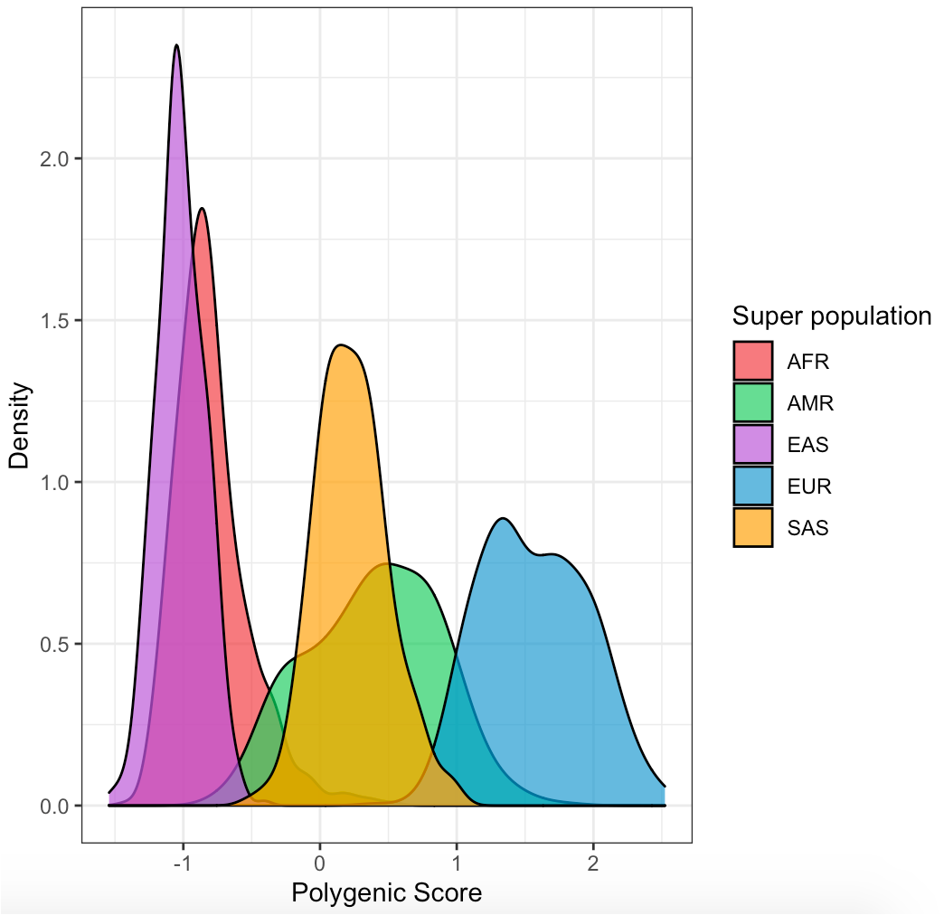
Visualize distribution of PRS in each population
# Libraries
library(ggplot2)
library(dplyr)

data <- read.csv("combine_profil_w_pop.txt", sep=" ")

data$SCORE_Z <- (data$SCORE-mean(data$SCORE))/sd(data$SCORE)

ggplot(data, aes(x=data$SCORE_Z, group=data$super_pop, fill=data$super_pop)) +
  geom_density(adjust=1.25, alpha=.7) +
  scale_fill_manual(values=c("brown2","springgreen3","mediumorchid","deepskyblue3","orange"))+
  labs(x = "Polygenic Score", y = "Density", fill = "Super population")+
  theme_bw() +
  theme(plot.title = element_text(hjust = 0.5))